AI Tools for Journalism

Jonathan Soma / js4571@columbia.edu / @dangerscarf

Abraji Conference 2023

🇧🇷 Auto-generated Portuguese translation can be found here: Versão em português

🕹️ GitHub repo can be found at https://github.com/jsoma/2023-abraji-ai-workshop

💻 Run this notebook as a live programming exercise here on Google Colab. Use shift+enter or the ▶️ button to run the code.

This web page was made from a Jupyter notebook! To see how I made it, see this tutorial about Quarto.

Introduction

Welcome to the page for my 2023 Abraji Data Sunday session!

This talk hopes to be as an introduction to a few key concepts to understanding artifical intelligence and machine learning. The biggest lessons to take away from this is what does AI people mean when they talk about “models,” and what are some things these models might be able to do? We focus on journalism, but I throw in a few options, too.

On this page you can find:

• Working code snippets for everything in my talk
• More in-depth information about each topic covered
• Links to AI-driven journalism projects
• Links to tutorials I’ve written on other topics
• Useful or neat things I didn’t cover in my talk.

Models

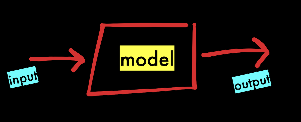
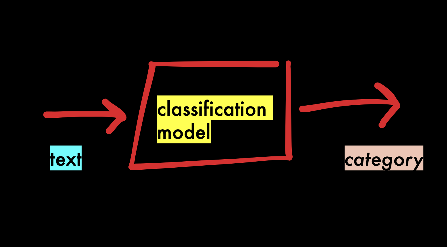
Models are what AI and machine learning are both based on. You have probably heard of some:

• Text models: GPT-2, GPT-3, GPT-3.5-turbo, GPT-4, Bard, Claude, LLaMa
• Image models: Stable Diffusion, Midjourney, DALL-E 2, Imagen

You give them an input, they give you an output. It sounds like a silly definition, but it’s true!

How models work

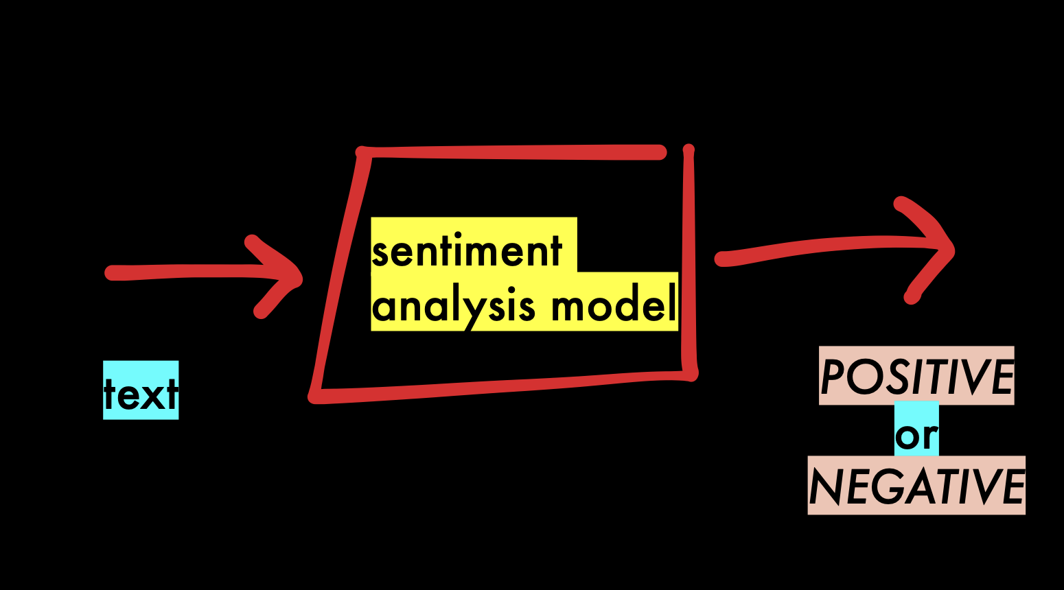
There are several major categories of models.

• Models that are trained on small amounts of data, just for one job
• Models that are trained on large amounts of data, then fine-tuned for one job
• Models that are trained on HUGE amounts of data and can already do everything

Classification

Sentiment analysis

Sentiment analysis says whether something is positive or negative. If we wanted to change the image above to reflect the specific knowledge of this model, it might look like this:

A sentiment analysis model

Let’s try sentiment analysis! Here is a small example, using the distilbert-base-uncased-finetuned-sst-2-english.

# First we'll install the "transformers" library from Hugging Face
!pip install -q --upgrade transformers

[notice] A new release of pip available: 22.3.1 -> 23.1.2
[notice] To update, run: python -m pip install --upgrade pip

from transformers import pipeline

sentiment_pipeline = pipeline("sentiment-analysis",
                             model="distilbert-base-uncased-finetuned-sst-2-english")
data = ["I enjoyed eating the sandwich"]

sentiment_pipeline(data)

[{'label': 'POSITIVE', 'score': 0.9996883869171143}]

This tells us that the sentence “I enjoyed eating my sandwich” is POSITIVE, and with a score of 0.999 which means the model is very certain.

Models are not perfect, and they only know what they know. If we read the details of the model we learn it is based on English. Because of this fact, how does it do if we try to use it on Portuguese text?

sentiment_pipeline = pipeline("sentiment-analysis",
                             model="distilbert-base-uncased-finetuned-sst-2-english")
data = ["Gostei de comer o sanduíche"]

sentiment_pipeline(data)

[{'label': 'POSITIVE', 'score': 0.5782410502433777}]

The model says this sentence is POSITIVE, but it is much less certain - 0.578. This feels like it isn’t working so well, but fortunately it’s easy to do better.

If we want to use Portuguese, we probably need a multi-lingual model. We could also find a model that only knows Portuguese, but it’s probably easier to find a model that speaks many languages and includes Portuguese.

We use the Hugging Face website to find one that looks promising:

Searching the Hugging Face model hub

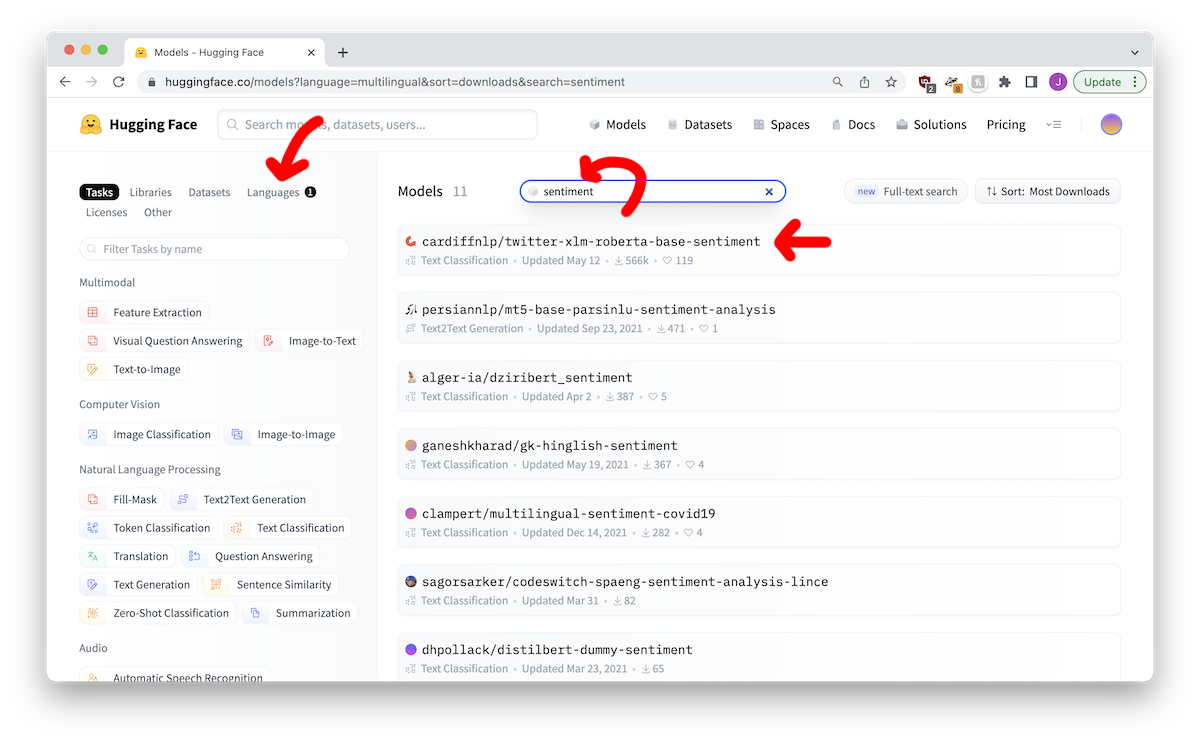
We can read details here, which includes this paragraph:

This is a multilingual XLM-roBERTa-base model trained on ~198M tweets and finetuned for sentiment analysis. The sentiment fine-tuning was done on 8 languages (Ar, En, Fr, De, Hi, It, Sp, Pt) but it can be used for more languages (see paper for details).

We don’t know what many of those terms mean, but Pt is Portuguese, so it sounds good to me!

To use this new model, which we just replace model="..." in our previous code with the new model’s name. The pipeline will automatically download it from Hugging Face and use it to judge our text.

sentiment_pipeline = pipeline("sentiment-analysis",
                             model="cardiffnlp/twitter-xlm-roberta-base-sentiment")
data = ["Gostei de comer o sanduíche"]

sentiment_pipeline(data)

[{'label': 'positive', 'score': 0.8415056467056274}]

Wonderful! While 0.841 is not as high as 0.999, it’s definitely more certain about the text being positive than the English model was. So far we have learned:

• There isn’t just one “sentiment analysis” – different models give different results!
• Different models might perform better or worse at different tasks or languages

This is because they are trained or fine-tuned in different ways.

Training custom models

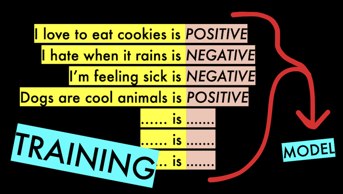
For sentiment analysis, the traditional way of training a model would be to show it examples of positive or negative sentences, and say “this one is positive!” or “this one is negative!” Over time the machine learns which words are associated with a positive sentence, and which are associated with a negative sentence.

Training a model

This doesn’t have to be about sentiment analysis, though! You can use this to put text into any type of categoy.

A model that puts content into different categories is called a classification model. A sentiment analysis model is just one simple example of a classification model.

Classification model

Classification models are common in investigative journalism when you have to analyze large amounts of data. You read several hundred documents, and mark the ones you are interested in. You use this to train a model, and the model then reads the rest for you, marking the interesting ones.

For example, the Washington Post had a model read thousands of app store reviews to find ones about unwanted sexual behavior on random chat apps. You can see a technical writeup I made of it here.

Another example, the LA Times used a classifier to examine crimes that were classified as either minor or serious, and determined the Los Angeles Police Department was misclassifying crimes. You can find my walkthroughs of that here or here.

One problem with these models is it is difficult for them to learn words as easily as people. For example, the words below all relate to the same action, but a classifier might see them all as very different words.

• Fish, fishes, fishing, fished
• correr, correndo, correu, correm

You can use stemming and lemmatization to fix the problem, but there are easier ways!

Fine-tuned models

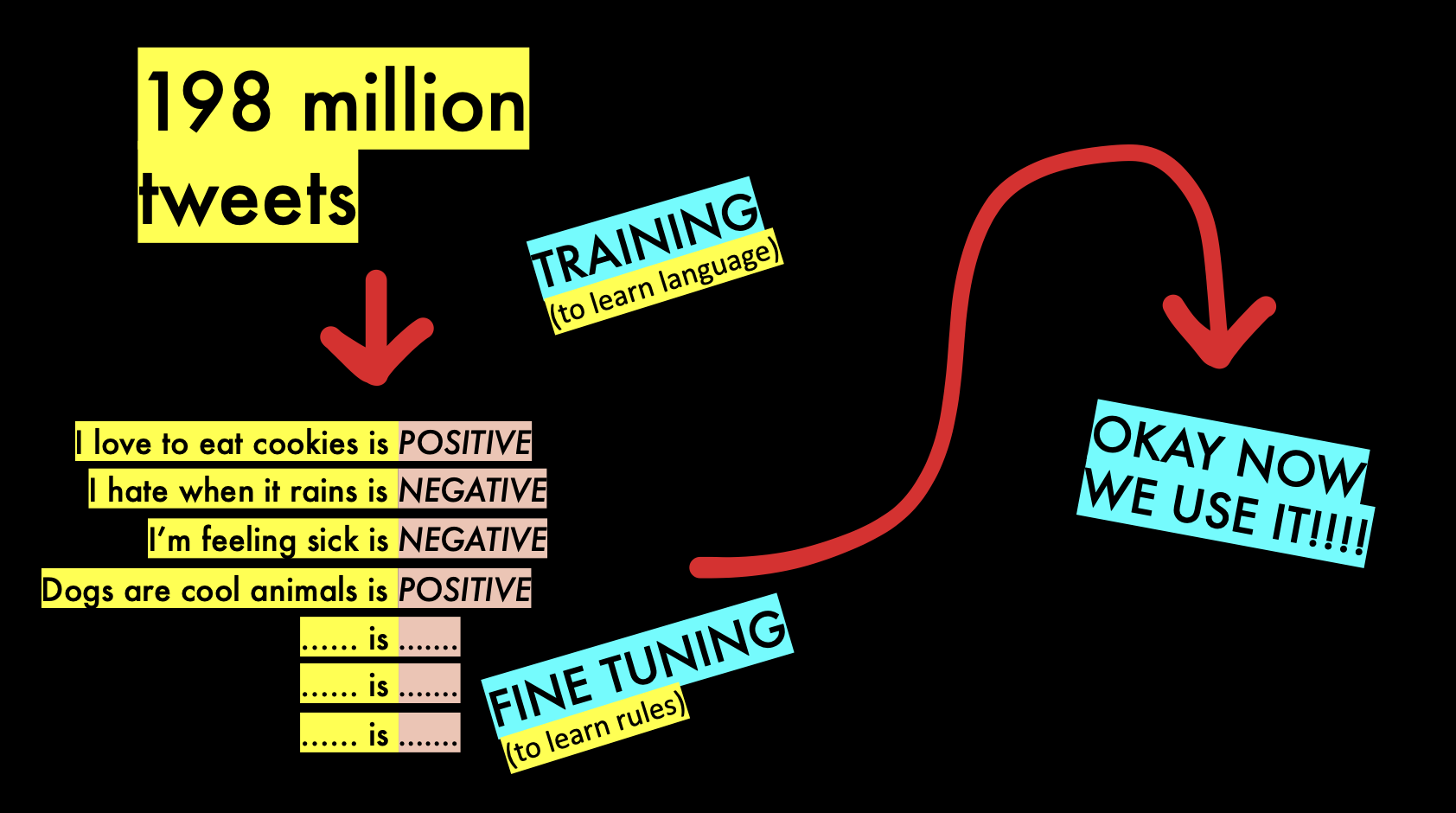
Instead of having a model learn language from zero, you can also use a pre-built model that knows a little language, then provide it a little extra information to make it good at the job you want it to do. It’s like hiring a teenager and teaching them to understand your text instead of hiring a baby that has never looked at a book before! This approach is called “fine tuning.”

For example, we can look at the details for the cardiffnlp/twitter-xlm-roberta-base-sentiment model we used before:

This is a multilingual XLM-roBERTa-base model trained on ~198M tweets and finetuned for sentiment analysis. The sentiment fine-tuning was done on 8 languages (Ar, En, Fr, De, Hi, It, Sp, Pt) but it can be used for more languages (see paper for details).

It read almost 200 million tweets to learn how the language in tweets works, then it was taught positive and negative sentiment afterwards. These models almost always perform better than the small custom models from the previous section.

fine-tuned model flow

To make a fine-tuned model, you can use the Hugging Face AutoTrainer to make it very easily. You upload a spreadsheet of your marked dataset, then it fine-tunes several models for you, and shows you the one that performed the best.

For example, this is a fine-tuned model I made for the Washington Post comments project. You can use it exactly like the sentiment analysis one! Let’s try it with two sentences:

sentiment_pipeline = pipeline(model="wendys-llc/creepy-wapo")
data = [
    "I love the app, talking to people is fun",
    "Be careful talking to men, they all want nudes :("
]

sentiment_pipeline(data)

[{'label': '0.0', 'score': 0.998849630355835},
 {'label': '1.0', 'score': 0.8436580300331116}]

You can see the first one is marked 0 (not creepy) and the second is marked 1 (creepy behavior). They also get a score as to how confident the model is that it’s making an accurate decision.

This model is based on a fine-tuned version of DeBERTa, a language model from Microsoft. You don’t have to pick the model: Hugging Face automatically fine-tunes five different language models for you and you can pick the best-performing one!

Large language models

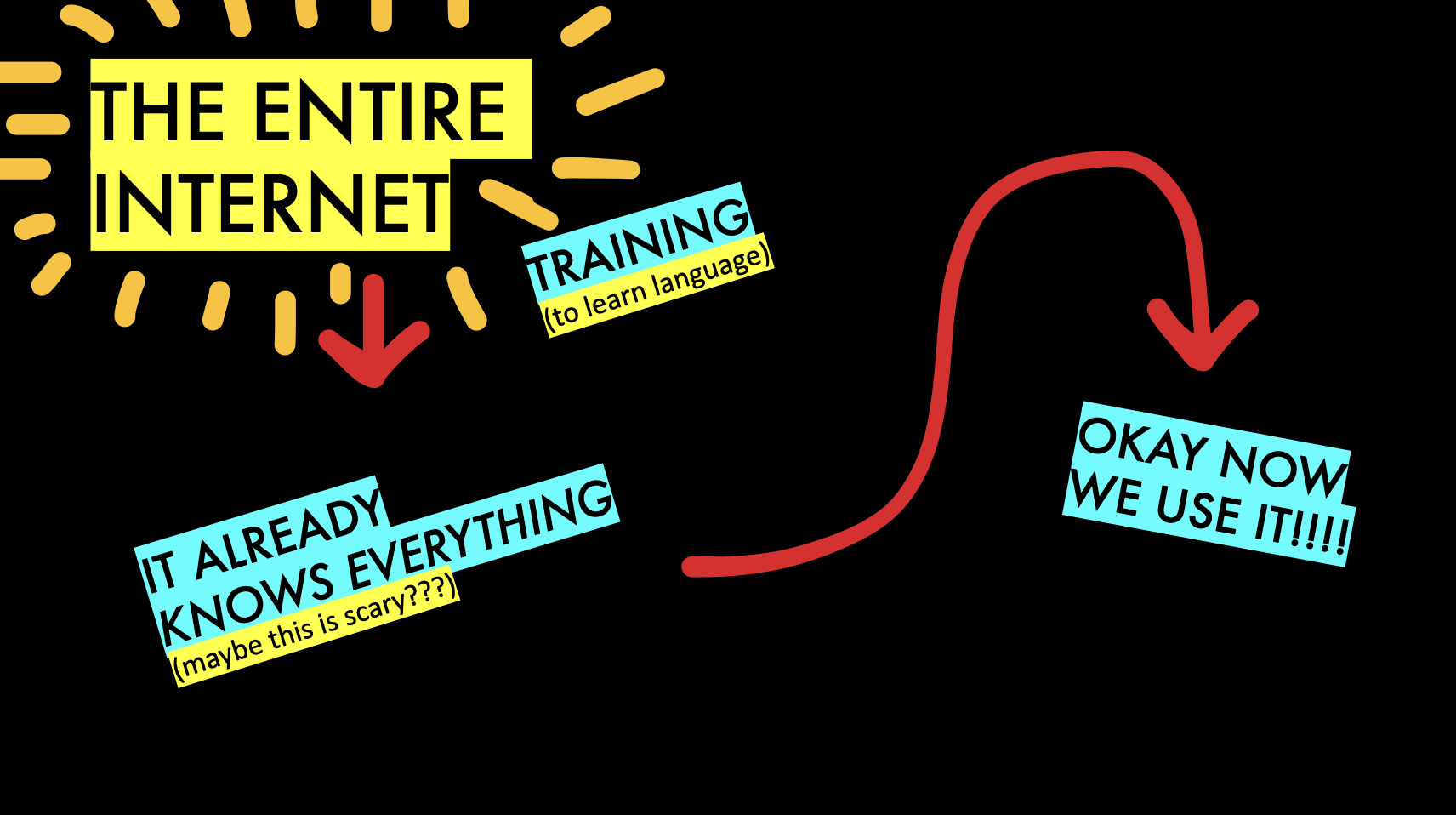
Large language models have changed everything! They are “large” because they know a lot more than previous models, and can do many tasks without fine tuning. They’ve read so much of the internet that they automatically know what positive and negative statements are!

large language model flow

You might be familiar with using ChatGPT to talk to the GPT model, but you can also use it in Python through an API. You need to register for an API key for the code below to work.

I personally like to use tools like GPT with Langchain, a library that makes working with large language models a little easier. After you set up an API key, you then need to install the libraries for both openai and langchain.

!pip install -q --upgrade openai langchain

from langchain.chat_models import ChatOpenAI

# You'll need your own OpenAI GPT API key! This one was mine,
# but I've deactivated it so I can publish this.
API_KEY = "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"

llm = ChatOpenAI(openai_api_key=API_KEY, model_name="gpt-3.5-turbo")

response = llm.predict("Give me a recipe for chocolate-chip cookies")
print(response)

Sure! Here's a classic recipe for chocolate chip cookies:

Ingredients:
- 1 cup unsalted butter, softened
- 1 cup granulated sugar
- 1 cup packed brown sugar
- 2 large eggs
- 1 teaspoon vanilla extract
- 3 cups all-purpose flour
- 1 teaspoon baking soda
- 1/2 teaspoon salt
- 2 cups chocolate chips

Instructions:
1. Preheat your oven to 375°F (190°C). Line a baking sheet with parchment paper or silicone baking mat.

2. In a large mixing bowl, cream together the softened butter, granulated sugar, and brown sugar until light and fluffy.

3. Beat in the eggs, one at a time, followed by the vanilla extract. Mix well after each addition.

4. In a separate bowl, whisk together the flour, baking soda, and salt. Gradually add the dry ingredients to the wet ingredients and mix until just combined. Avoid overmixing.

5. Stir in the chocolate chips until evenly distributed throughout the dough.

6. Using a cookie scoop or a tablespoon, drop rounded balls of dough onto the prepared baking sheet, spacing them about 2 inches apart.

7. Bake in the preheated oven for 9-11 minutes, or until the cookies are golden brown around the edges. The centers may still appear slightly undercooked, but they will firm up as they cool.

8. Allow the cookies to cool on the baking sheet for 5 minutes, then transfer them to a wire rack to cool completely.

9. Enjoy your homemade chocolate chip cookies with a glass of milk or as a sweet treat!

Note: Feel free to customize your cookies by adding chopped nuts, using different types of chocolate chips, or incorporating other mix-ins like shredded coconut or dried fruit.

Zero-shot classification

Now that we can interact with GPT using Python, we can create a classifier without training or fine-tuning at all. We just need to give GPT the text and tell it what categories we are looking for. This is called zero-shot classification because it takes zero examples for the classifier to learn.

For example, maybe I want to classify the text of a bill.

prompt = """
Categorize the following text as being about ENVIRONMENT, GUN CONTROL,
or IMMIGRATION. Respond with only the category.

Text: A Bill to Regulate the Sulfur Emissions of Coal-Fired Energy
Plants in the State of New York.
"""

response = llm.predict(prompt)
print(response)

ENVIRONMENT

It’s so easy!!! You can also make use of Python’s .format method to make things even simpler if you want to make a lot of requests.

template = """
Categorize the following text as being about ENVIRONMENT, GUN CONTROL,
or IMMIGRATION. Respond with only the category.

Text: {bill_text}
"""

print(template.format(bill_text="This fills in the spot in the template"))

Categorize the following text as being about ENVIRONMENT, GUN CONTROL,
or IMMIGRATION. Respond with only the category.

Text: This fills in the spot in the template

template = """
Categorize the following text as being about ENVIRONMENT, GUN CONTROL,
or IMMIGRATION. Respond with only the category.

Text: {bill_text}
"""

bills = [
    "A Bill to Allow Additional Refugees In Upstate New York",
    "A Bill to Close Down Coal-fired Power Plants",
    "A Bill to Banning Assault Rifles at Public Events"
]

for bill in bills:
    prompt = template.format(bill_text=bill)
    response = llm.predict(prompt)
    print(bill, "is", response)

A Bill to Allow Additional Refugees In Upstate New York is IMMIGRATION
A Bill to Close Down Coal-fired Power Plants is ENVIRONMENT
A Bill to Banning Assault Rifles at Public Events is GUN CONTROL

There is also few-shot classification which provides several examples to the LLM when you want to classify something. For example, I might provide two or three tricky situations or edge cases in the prompt so the classifier knows what I really want.

Named Entity Recognition

Named entity recognition is the ability to recognize people, places, companies, and other things inside of your text. It’s like classification, but for parts of a text. It’s often used to extract the names of people from documents.

A use case for NER might be assuring gender parity for sources in your publication. You can read here about wonderful work being done in this field by La Nación.

Using spaCy

Traditionally, you would use a tool like spaCy to do named entity recognition. You’d probably still do that, honestly, it works pretty well and (unlike GPT models) it’s free!

If you’ve ever heard of NLTK, a common text analysis library, spaCy is the cool, fun, modern version.

We’ll start by installing spaCy and downloading two models: one is a medium-sized English model, and the other is focused on Portuguese. You can find these models on the spaCy usage page.

!pip install -q spacy
!python -m spacy download en_core_web_md
!python -m spacy download pt_core_news_lg

Now let’s try them both out. We’ll start with en_core_web_md for English text.

import spacy

nlp = spacy.load("en_core_web_md")
text = "Hi, I'm Jonathan Soma, and I'm giving this talk at the Abraji Conference in Sāo Paulo."
doc = nlp(text)

for ent in doc.ents:
    print(ent.text, ent.label_)

Jonathan Soma PERSON
the Abraji Conference FAC
Sāo Paulo GPE

Does it work as well for Portuguese?

import spacy

nlp = spacy.load("en_core_web_md")
text = "Olá, eu sou Jonathan Soma e estou dando esta palestra na Congresso da Abraji em São Paulo"
doc = nlp(text)

for ent in doc.ents:
    print(ent.text, ent.label_)

Jonathan Soma PERSON
Congresso ORG

Maybe we can also try the specific Portuguese model to see if it performs any better.

import spacy

nlp = spacy.load("pt_core_news_lg")
text = "Olá, eu sou Jonathan Soma e estou dando esta palestra na Congresso da Abraji em São Paulo"
doc = nlp(text)

for ent in doc.ents:
    print(ent.text, ent.label_)

Jonathan Soma PER
Congresso da Abraji MISC
São Paulo LOC

Using an LLM

In the same way we can use an LLM for classification, we can also use it for named entity recognition!

from langchain.chat_models import ChatOpenAI

# You'll need your own OpenAI GPT API key! This one was mine,
# but I've deactivated it so I can publish this.
API_KEY = "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"

llm = ChatOpenAI(openai_api_key=API_KEY, model_name="gpt-3.5-turbo")

prompt = """
List the named entities in the text below. Use a comma to
separate the entity and the type of entity. Valid entity
types are PERSON, EVENT, ORGANIZATION, and LOCATION.

Text: Hi, I'm Jonathan Soma, and I'm giving this talk at the Abraji Conference in Sāo Paulo.
"""

response = llm.predict(prompt)
print(response)

Jonathan Soma (PERSON), Abraji Conference (EVENT), Sāo Paulo (LOCATION)

I didn’t really want those parentheses, but it’s pretty good! Let’s see how it works with Portuguese:

prompt = """
List the named entities in the text below. Use a comma to
separate the entity and the type of entity. Valid entity
types are PERSON, EVENT, ORGANIZATION, and LOCATION.

Text: Olá, eu sou Jonathan Soma e estou dando esta palestra na Congresso da Abraji em São Paulo.
"""

response = llm.predict(prompt)
print(response)

Jonathan Soma - PERSON
Congresso da Abraji - EVENT
São Paulo - LOCATION

Notice it didn’t listen to my instructions perfectly! Instead of using a comma to separate the entity and type, it used a hyphen instead. Large language models can be slightly unpredictabe, and you often need to be aggressive to keep it doing what you want.

Document search and similarity

Investigations often involve combing through documents that are in different languages. How Quartz used AI to sort through the Luanda Leaks gives a good background on the difficulty involved in the process!

!pip install -q sentence-transformers sentencepiece

In the code below we generate text embeddings. You can read a writeup of mine about embeddings here, but the short description is that words and sentences are turned into concepts. Instead of matches based on exact words, or even fish-fishes-fishing, you can match with general ideas.

As a bonus: if you use a multi-lingual model, the same concepts can be matched even if the documents are in different languages!

from sentence_transformers import SentenceTransformer
sentences = ["This is an example sentence"]

model = SentenceTransformer('sentence-transformers/all-MiniLM-L6-v2')
embeddings = model.encode(sentences)
print(embeddings[0][:50])

[ 0.0676569   0.06349581  0.0487131   0.07930496  0.03744796  0.00265277
  0.03937485 -0.00709837  0.0593615   0.03153696  0.06009803 -0.05290522
  0.04060676 -0.02593078  0.02984274  0.00112689  0.07351495 -0.05038185
 -0.12238666  0.02370274  0.02972649  0.04247681  0.0256338   0.00199517
 -0.05691912 -0.02715985 -0.03290359  0.06602488  0.11900704 -0.04587924
 -0.07262138 -0.03258408  0.05234135  0.04505523  0.00825302  0.03670237
 -0.01394151  0.06539196 -0.02642729  0.00020634 -0.01366437 -0.03628108
 -0.0195043  -0.02897387  0.03942709 -0.08840913  0.00262434  0.01367143
  0.04830637 -0.03115652]

Those numbers above might look awful, but they are how computers think about concepts! If two pieces of text have similar numbers, they’re probably about the same thing (…kind of).

A visual representation of word embeddings

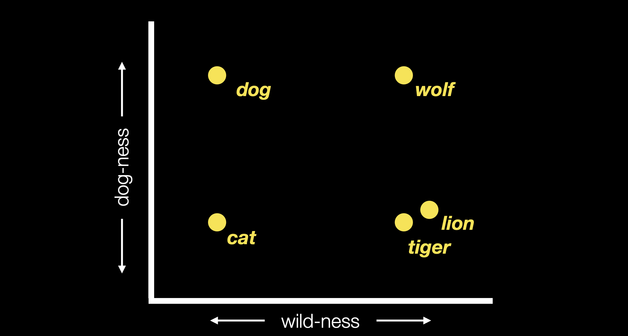
Let’s look at a better example of how a single-language and multi-language embedding might make sentences more or less similar to each other.

import pandas as pd

sentences = [
    "Molly ate a fish",
    "Jen consumed a carp",
    "I would like to sell you a house",
    "Я пытаюсь купить дачу", # I'm trying to buy a summer home
    "J'aimerais vous louer un grand appartement", # I would like to rent a large apartment to you
    "This is a wonderful investment opportunity",
    "Это прекрасная возможность для инвестиций", # investment opportunity
    "C'est une merveilleuse opportunité d'investissement", # investment opportunity
    "これは素晴らしい投資機会です", # investment opportunity
    "野球はあなたが思うよりも面白いことがあります", # baseball can be more interesting than you think
    "Baseball can be interesting than you'd think"
]

model = SentenceTransformer('sentence-transformers/all-MiniLM-L6-v2')
embeddings = model.encode(sentences)

from sklearn.metrics.pairwise import cosine_similarity

# Compute similarities exactly the same as we did before!
similarities = cosine_similarity(embeddings)

# Turn into a dataframe
pd.DataFrame(similarities,
            index=sentences,
            columns=sentences) \
            .style \
            .background_gradient(axis=None)

	Molly ate a fish	Jen consumed a carp	I would like to sell you a house	Я пытаюсь купить дачу	J'aimerais vous louer un grand appartement	This is a wonderful investment opportunity	Это прекрасная возможность для инвестиций	C'est une merveilleuse opportunité d'investissement	これは素晴らしい投資機会です	野球はあなたが思うよりも面白いことがあります	Baseball can be interesting than you'd think
Molly ate a fish	1.000000	0.526053	0.025476	0.098335	0.020435	-0.065293	0.035801	-0.062506	0.027358	0.017622	0.023445
Jen consumed a carp	0.526053	1.000000	0.044178	0.035044	-0.018194	-0.004438	-0.078566	-0.011418	0.090357	0.131507	0.016100
I would like to sell you a house	0.025476	0.044178	1.000000	0.154773	0.083555	0.386736	0.017175	-0.006744	0.010857	0.025510	0.006353
Я пытаюсь купить дачу	0.098335	0.035044	0.154773	1.000000	0.159519	0.064379	0.462397	0.092110	0.314708	0.327675	-0.119607
J'aimerais vous louer un grand appartement	0.020435	-0.018194	0.083555	0.159519	1.000000	0.032253	0.365505	0.566635	0.172406	0.110118	-0.013743
This is a wonderful investment opportunity	-0.065293	-0.004438	0.386736	0.064379	0.032253	1.000000	-0.030322	0.212230	0.023889	-0.002844	0.112804
Это прекрасная возможность для инвестиций	0.035801	-0.078566	0.017175	0.462397	0.365505	-0.030322	1.000000	0.282414	0.267571	0.285873	-0.040309
C'est une merveilleuse opportunité d'investissement	-0.062506	-0.011418	-0.006744	0.092110	0.566635	0.212230	0.282414	1.000000	0.292651	0.187989	0.006793
これは素晴らしい投資機会です	0.027358	0.090357	0.010857	0.314708	0.172406	0.023889	0.267571	0.292651	1.000000	0.577265	-0.100630
野球はあなたが思うよりも面白いことがあります	0.017622	0.131507	0.025510	0.327675	0.110118	-0.002844	0.285873	0.187989	0.577265	1.000000	-0.098722
Baseball can be interesting than you'd think	0.023445	0.016100	0.006353	-0.119607	-0.013743	0.112804	-0.040309	0.006793	-0.100630	-0.098722	1.000000

Sentence that are about the same thing don’t match, just because they’re in different languages! Don’t worry, there are some pretrained multilingual models, let’s see how much better that one looks.

model = SentenceTransformer('sentence-transformers/distiluse-base-multilingual-cased-v2')
embeddings = model.encode(sentences)

from sklearn.metrics.pairwise import cosine_similarity

# Compute similarities exactly the same as we did before!
similarities = cosine_similarity(embeddings)

# Turn into a dataframe
pd.DataFrame(similarities,
            index=sentences,
            columns=sentences) \
            .style \
            .background_gradient(axis=None)

	Molly ate a fish	Jen consumed a carp	I would like to sell you a house	Я пытаюсь купить дачу	J'aimerais vous louer un grand appartement	This is a wonderful investment opportunity	Это прекрасная возможность для инвестиций	C'est une merveilleuse opportunité d'investissement	これは素晴らしい投資機会です	野球はあなたが思うよりも面白いことがあります	Baseball can be interesting than you'd think
Molly ate a fish	1.000000	0.358347	0.058340	0.145439	-0.024103	-0.070145	-0.075333	-0.073496	-0.111467	-0.025614	0.001549
Jen consumed a carp	0.358347	1.000000	0.059195	0.190241	-0.001941	-0.024359	-0.024816	-0.023295	-0.087019	0.040799	0.067243
I would like to sell you a house	0.058340	0.059195	1.000000	0.418692	0.642746	0.081795	0.118611	0.067805	0.042560	0.144491	0.139300
Я пытаюсь купить дачу	0.145439	0.190241	0.418692	1.000000	0.351605	0.120679	0.184644	0.144633	0.115598	0.050505	0.046084
J'aimerais vous louer un grand appartement	-0.024103	-0.001941	0.642746	0.351605	1.000000	0.203307	0.238716	0.204762	0.195163	0.201317	0.151998
This is a wonderful investment opportunity	-0.070145	-0.024359	0.081795	0.120679	0.203307	1.000000	0.953561	0.964282	0.945246	0.062618	0.133220
Это прекрасная возможность для инвестиций	-0.075333	-0.024816	0.118611	0.184644	0.238716	0.953561	1.000000	0.968368	0.944719	0.084221	0.136699
C'est une merveilleuse opportunité d'investissement	-0.073496	-0.023295	0.067805	0.144633	0.204762	0.964282	0.968368	1.000000	0.959357	0.086458	0.146568
これは素晴らしい投資機会です	-0.111467	-0.087019	0.042560	0.115598	0.195163	0.945246	0.944719	0.959357	1.000000	0.091451	0.115392
野球はあなたが思うよりも面白いことがあります	-0.025614	0.040799	0.144491	0.050505	0.201317	0.062618	0.084221	0.086458	0.091451	1.000000	0.839617
Baseball can be interesting than you'd think	0.001549	0.067243	0.139300	0.046084	0.151998	0.133220	0.136699	0.146568	0.115392	0.839617	1.000000

If you’re interested in how this might work with GPT or other large language model, you might want to check out this GitHub repo.

Summarization

I personally think it’s best to keep LLM-generated content to be reporter-facing, not user-facing. A journalist’s only job is to be accurate, but LLMs love to make things up. The NYT recently said AI takes too much time to fact-check to be useful and a Danish newsroom found LLM-generated article summaries inadequate around half the time:

I hope to reach a point where we can trust the summaries and publish them directly without a human in the loop, but we’re not there yet. In the rest of this post I examine the quality of these AI-generated summaries and the ongoing need for a human in the loop.

But if you’re interested in how that might work, we can use Langchain for simple document summarization. In this example, we’re going to summarize a Hungarian folktale into English.

We’ll start by reading in the text.

from langchain.document_loaders import TextLoader
from langchain.text_splitter import RecursiveCharacterTextSplitter

loader = TextLoader('folktale.txt')
documents = loader.load()

text_splitter = RecursiveCharacterTextSplitter(chunk_size=2500)
docs = text_splitter.split_documents(documents)
len(docs)

20

Because of token limits (see below), we can only send around 4000 tokens (3000 words) to the LLM at a time. As a result, we need to split the document into 2500-token chunks (around 1900 words each) to send individually. Later on we’ll combine the summaries into one larger summary.

Let’s look at the first 500 characters of our first document.

print(docs[0].page_content[:500])

RÁADÓ ÉS ANYICSKA.
Egyszer, hol volt – hol nem volt, volt a világon egy király, a ki teljeséletében mindig a háborúban, harczban lakott. Már kilencz esztendő óta aháza tájékán se’ volt, azt se’ tudta hogy mije van otthon. Elhatároztahát hogy már csak akárhogy – mint teszi szerét, de haza megy, feliratjamindenét az utolsó tűig, hogy legalább tudja, mit keresett kilenczesztendő óta.
Békét kötött hát az ellenséggel három hónapra, avval elindult hazafelé.Mikor hazaért, összegyűjtötte a sok herczeget

I don’t know Hungarian, but it looks good to me! Now we connect to our good friend GPT…

from langchain.chat_models import ChatOpenAI

# You'll need your own OpenAI GPT API key! This one was mine,
# but I've deactivated it so I can publish this.
API_KEY = "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"

# Connect to the LLM
llm = ChatOpenAI(openai_api_key=API_KEY,
                 model_name="gpt-3.5-turbo",
                 temperature=0)

Summarization of long documents has a lot of little tricks to make it successful. In this case we’re going to use a custom prompt: while it isn’t necessary, I think it’s probably better to have more control. We also want to make sure the summary is in English instead of Hungarian.

You can see a few other approaches on this awful Langchain page – some of them don’t work, or they perfom the same task in different ways without explaining the benefits of one or another, or have other problems.

from langchain import PromptTemplate
from langchain.chains.summarize import load_summarize_chain

prompt_template = """Write a concise summary of the following text. Since it's a folktale, it's
important that the summary include the challenges the main character might face.


TEXT: {text}


CONCISE SUMMARY IN ENGLISH:"""
PROMPT = PromptTemplate(template=prompt_template, input_variables=["text"])
chain = load_summarize_chain(llm,
                             chain_type="map_reduce",
                             return_intermediate_steps=True,
                             map_prompt=PROMPT,
                             combine_prompt=PROMPT)

result = chain({"input_documents": docs}, return_only_outputs=True)

It takes a while to run this step, because it has to summarize each and every one of the chunks, then summarize the summaries. If we were using GPT-4 with larger token limits we would be able to do this more quickly, even if it did cost more.

Let’s look at the output!

print(result['output_text'])

The text is a folktale about a king who returns home from war and learns that he has a son he didn't know about. The son, named Raadó, is taken by a powerful fairy king in exchange for the information. Raadó follows the instructions of a beautiful fairy to win the love of a princess and prove himself to the fairy king. He faces challenges in keeping their love a secret and proving his abilities to the queen. Raadó also faces challenges in completing tasks given to him by the king, such as clearing a forest and riding fiery horses. He is able to overcome these challenges with the help of magical assistance and his own determination. The story ends with Raadó and the princess being reunited and living happily ever after.

Seems fine, but remember the link from before: most article summaries didn’t pass muster once they were reviewed!.

Limitations of large language models

The knowledge cutoff is a big one, where they only know what’s in their training data. In the case of GPT, it stopped getting new information in September 2021.

The token limit is another issue, where you can only provide so much information to the AI tool at a time, usually several thousand words. Newer language models have larger token limits – there is a version of GPT-4 that allows 32k tokens, which is around 24,000 words – and AnthropicAI’s Claude has a 100k context window. This is definitely one area where providers are competing!

There are ways to get around these problems, which you can see some details of in my Media Party Chicago 2023 talk. Technically speaking it’s called “in-context learning with semantic search,” and it’s the baseline of all of the “chat with your PDF” kind of tools you might have seen.

The biggest limitation of an LLM is hallucinations, where it will just make things up! My two suggestions for this are don’t use LLMs as a knowledge base and always fact-check. Even simple tasks are prone to hallucinations: a Danish newspaper found GPT-generated article summaries often contained information not in the original piece.

Image-based models

Image-based models can allow you to do things like research using aerial and satellite photography, as was done in Leprosy of the Land when computer vision could detect illegal amber mines.

You can view code samples and get more ideas by browsing the Hugging Face website.

Image classification

Leprosy of the Land was an image classification problem, which is practically the same as text classification! If you wanted to do a similar problem, you can similarly train a custom model or fine-tune an existing image model.

To fine-tune an existing image model, I again recommend Hugging Face AutoTrain. You upload folders with several examples of each category or class you’re looking for, and it automatically creates a model for you.

You can see a tutorial I gave on this (with data) here on GitHub, or the completed model here.

We’ll start by opening our image. Those little dots are amber mines!

# Pillow is a Python image processing library
!pip install --quiet pillow

from PIL import Image

image = Image.open("amber-example-1.png")
image

Now we will load in our model, use a “feature extractor” to convert our image to the format the model wants, and then ask it whether the image contains amber mines or not.

from transformers import AutoFeatureExtractor, AutoModelForImageClassification

# Load our model
extractor = AutoFeatureExtractor.from_pretrained("wendys-llc/autotrain-amber-mines-42327108538")
model = AutoModelForImageClassification.from_pretrained("wendys-llc/autotrain-amber-mines-42327108538")

# Convert to encoding the model understands
encoding = extractor(image, return_tensors="pt")

# Send the encoded image to the model, get the outputs
outputs = model(**encoding)
logits = outputs.logits

# Find what class (what category) it predicted
predicted_class_idx = logits.argmax(-1).item()

# Print out the answer
print("Predicted class:", model.config.id2label[predicted_class_idx])

Predicted class: positive

Success! It took a few more lines of code than the text-based examples above, but it isn’t too bad. There are a good number of technical pieces in there – tensors, logits, argmax – but you don’t 100% need to know how they work as long as you just use the same code all of the time. If you’re interested in getting deeper into machine learning, though, it’s probably good to read up on them.

While the amber mines example is a fine-tuned model, we can also use zero-shot image classification, just like we did with the text up above. To see an example of of how zero-shot image classification might work, select one of the images below. You can also read up on the model this app uses.

Semantic segmentation

Another great tool to use with images is semantic segmentation. This allows you to classify different pixels in an image.

This is common for using aerial or satellite photography to determine land use, finding asphalt/roads, or greenery or crops. For example, you might look at all of the neighborhoods in a city and see which one has the most coverage by trees, or inspect deforestation using Global Forest Watch.

You can learn more about that at Normal AI. To use the example below, scroll down and click one of the example images.

Object detection

Object detection might be the easiest to explain: it detects objects in images! While object detection is easy to explain, I find it is difficult to find journalistic use cases for it. It has potential for face detection or finding cars or trucks in photographs, but I’m not sure of when that’s been used for journalism.

It also doesn’t always do a perfect job: it’s pre-trained with some number of existing objects, but sometimes you want specific objects that the pre-trained models don’t know about.

You can learn more about that at Normal AI. To use the example below, scroll down and click one of the example images.

Image generation

While DALL-E 2 was definitely the most popular image generation tool, I strongly recommend checking out Midjourney instead. It’s a little more complicated to use than DALL-E – it requires logging into their Discord server, a kind of chat room – and costs $8/month, but it’s worth a short subscription to see how well it performs!

Audio models

Whisper is a model that transcribes audio. People have generally been very impressed by it!

The example below uses a large, more skillful version of the model, and it should be able to work in both English and non-English languages. I recommend using the “Record from microphone” and recording a snippet of yourself speaking.

Finding more models and expanding your skills

I recommend browsing the Hugging Face models page or their spaces page, which shows examples of small projects people have made. You can also keep your eyes and ears open – when you hear about fancy models being released or available, check and see if they’re on Hugging Face!

My old web site investigate.ai: Data science for journalists has a lage number of projects, but a number of them are built using “old” technology. They still work, but for example using a fine-tuned language model is probably a better route to text classification than the custom model I show you.

You can also keep up to date with AI by reading Jack Clark’s Import AI, a weekly newsletter. I hate newsletters but it’s pretty good!

If you’d like to get deeper into using LLMs as part of your workflow, learning how Langchain or Llama Index work could be a good investment. Langchain is probably more popular, but the examples are often confusing or have older, broken code. I also recommend taking a look at YouTube for both of those tools!

Contact me

Feel free to reach out – I’m more than happy to provide ideas, guidance, lectures, etc etc etc. You can find me via email at js4571@columbia.edu or on Twitter at @dangerscarf. I also run two data journalism programs at Columbia: the 12-month Data Journalism MS and the Lede Program, a summer intensive.